
Contents
Time series data occur almost everywhere. Much of the recent hype (mostly deserved) around deep learning architectures has been around the state-of-the-art performance produced in the fields of computer vision, natural language processing, and bioinformatics. Much of “deep learning” is a rebranding of neural networks. During my second year of graduate school, I became interested in applying machine learning to time series data which I planned to use as my dissertation topic. I ended up studying reinforcement learning in social graphs, but I’ll save that for another time. In this tutorial, I’ll discuss applying convolutional neural networks to time series data.
Convolutional Neural Networks
Convolutional Neural Networks (CNN) are biologically-inspired variants of MLPs. From Hubel and Wiesel’s early work on the cat’s visual cortex, we know the visual cortex contains a complex arrangement of cells. These cells are sensitive to small sub-regions of the visual field, called a receptive field. The sub-regions are tiled to cover the entire visual field. These cells act as local filters over the input space and are well-suited to exploit the strong spatially local correlation present in natural images.1
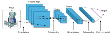
Typical CNN architecture
CNNs may be applied to multivariate time series. It can be useful to think of a time series as a one-dimensional image. You don’t need to use an image of the time series as input to the CNN! I’ve seen several papers which used this approach which seems weird, you just need to use a 1-dimensional convolutional layer instead of the typical 2-D layer. In the 1D domain, a convolution can be viewed as a filter, capable of removing outliers, filtering the data or acting as a feature detector, defined to respond maximally to specific temporal sequences within the filter length of the convolution.
To better understand this, consider the definition of a 1-D convolution.
There are two input signals, x and h and N is the length of h. The output vector is y, h is known as the kernel or convolution filter and x is the input data. The subscripts denote the nth element of the vector. Here is an example of how the convolution is calculated when h has three elements:
$$
\begin{aligned}
y_{0} & = h_{0} \cdot x_{0} \\
y_{1} & = h_{1} \cdot x_{0} + h_{0} \cdot x_{1} \\
y_{2} & = h_{2} \cdot x_{0} + h_{1} \cdot x_{1} + h_{0} \cdot x_{2} \\
y_{3} & = h_{2} \cdot x_{1} + h_{1} \cdot x_{2} + h_{0} \cdot x_{3} \\
\vdots
\end{aligned}
$$
The filter [\(h_2 h_1 h_0\)] is slid along the elements of x and at each step we multiply the elements and sum them: the result will be the corresponding element of the output y vector. Here is a concrete example:
$$
\begin{aligned}
x & = \left[
\begin{array}{c} 1 \, 2 \, 1 \, 3
\end{array}
\right]
\\
h & = \left[
\begin{array}{c}
2 \, 0 \, 1
\end{array}
\right]
\end{aligned}
\\
\begin{array}{c|cccccccc|r}
k & \it{0} & \it{0} & 1 & 2 & 1 & 3 & \it{0} & \it{0} & \it{y_{k}}\\
\hline
0 & 1 & 0 & 2 & & & & & & 2 \cdot 1 = 2\\
1 & & 1 & 0 & 2 & & & & & 2 \cdot 2 = 4\\
2 & & & 1 & 0 & 2 & & & & 2 \cdot 1 + 1 \cdot 1 = 3\\
3 & & & & 1 & 0 & 2 & & & 2 \cdot 3 + 1 \cdot 2 = 8\\
4 & & & & & 1 & 0 & 2 & & 1 \cdot 1 = 1\\
5 & & & & & & 1 & 0 & 2 & 1 \cdot 3 = 3\\
\end{array}
$$
It is easy to see that a simple moving average is a special case of a convolution using the following kernel:
$$
h = \left[
\begin{array}{c} \dfrac{1}{N} \, \dfrac{1}{N} \, ... \, \dfrac{1}{N}\, \dfrac{1}{N}\end{array}
\right]
$$
Hopefully, this gives some intuition as to what a one-dimensional convolution does. A 1-dimensional convolution applied to multiple input signals creates a linear combination of the filtered inputs at each time step.
Data
I’m going to use the UCI Machine Learning Human Activity Recognition dataset for this example. The dataset consists of sensor data recorded from 30 subjects performing activities of daily living, specifically, WALKING, WALKING_UPSTAIRS, WALKING_DOWNSTAIRS, SITTING, STANDING, LAYING. The data was collected from 30 individuals who wore a Samsung Galaxy S II on their waist. The sampling rate was 50Hz and sensor signals (accelerometer and gyroscope) were pre-processed by applying noise filters and then sampled in fixed-width sliding windows of 2.56 sec and 50% overlap (128 readings/window). If you don’t care about any of this and just want an input into your blackbox, we have 128 observations of a 9-dimensional time series with 6 unique classes.
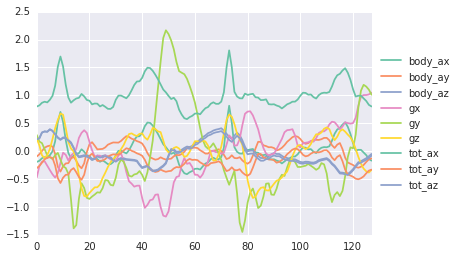
De-noised sensor data from mobile phone
Example
I’m a big fan of the neural networks library Keras. Keras can run on top of the deep learning libraries Theano and Tensorflow and makes prototyping neural networks very easy. Here I’ll use Keras to build a convolutional neural network to predict the activities from the sensor data provided by Human Activity Recognition dataset.
from keras.models import Sequential
from keras.layers.core import Dense, Dropout, Activation, Flat
from keras.layers.convolutional import Convolution1D, MaxPooling1D

#set parameters
batch_size = 50
nb_filter = 64 #number of features to learn
filter_length = 10 #number of time steps
hidden_dims = 250
nb_epoch = 50
n_sensors = 9
classes = 6
pool_length = 64
subsample_length = 2


model = Sequential()

model.add(Convolution1D(nb_filter=64,
                        filter_length=10,
                        subsample_length=subsample_length,
                        border_mode='same',input_shape=(128,9)))
# we use standard max pooling (halving the output of the previous layer):
model.add(MaxPooling1D(pool_length=pool_length))
# We flatten the output of the conv layer,
# so that we can add a vanilla dense layer:
model.add(Flatten())

model.add(Dense(hidden_dims))
model.add(Dense(classes))
model.add(Activation('softmax'))

model.compile(loss='categorical_crossentropy',optimizer='rmsprop')
model.fit(xtrain,ytrain,batch_size=batch_size,nb_epoch=nb_epoch,show_accuracy=True)
What is happening inside the network?
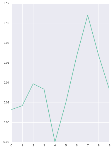
Here are a few examples of some well known filters from digital signal processing:
High and low pass filters remove certain frequencies from the original signal. You can think of the high-pass filter as removing any underlying trend in the signal and the low-pass filter as smoothing the signal to extract the trend.
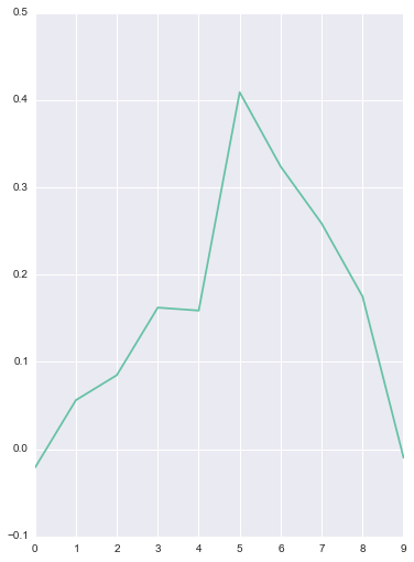
The derivative of an input signal can be approximated by convolving the derivative of a Gaussian Filter or by using a discrete derivative filter (as shown above). Since we typically use a max pooling layer after a convolutional layer, we are able to identify the maximum value of the derivative over the time interval of the input. Inverting attenuators flip the signal and enable us to extract minimum values of the signal’s derivative using a max pooling layer.
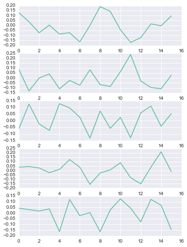
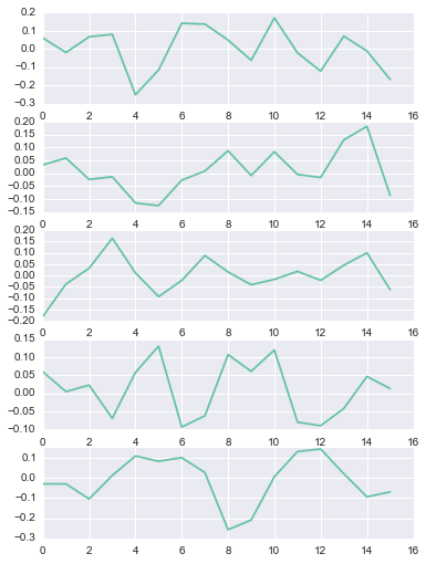
After training the model, we can look at some of the learned filters to get a sense of what types of features the CNN extracts.
The filter on the left is learned for the y-axis acceleration and looks very close to a derivative filter. The filter on the right is similar to a high-pass filter and was learned for the g1 gyroscope axis. Some of the other filters aren’t as obvious, however, it appears that many of the learned filters are similar to well known techniques from signal processing.
Images from https://www.dspguide.com
Results
Test set summary:
class   precision    recall  f1-score   support
0         0.98      0.92      0.95       496
1         0.95      0.94      0.94       471
2         0.89      1.00      0.94       420
3         0.86      0.92      0.89       491
4         0.96      0.87      0.91       532
5         1.00      1.00      1.00       537

total      0.94      0.94      0.94      2947
Training set summary:
class   precision   recall  f1-score   support

0         1.00      1.00      1.00      1226
1         1.00      1.00      1.00      1073
2         1.00      1.00      1.00       986
3         0.91      1.00      0.95      1286
4         1.00      0.91      0.95      1374
5         1.00      1.00      1.00      1407

total     0.98      0.98      0.98      7352
A 1-layer convolutional + max pooling neural network achieves 94% accuracy with somewhat arbitrary hyperparameters (I choose the parameters to help simplify the visualizations of each of the activations.) This is a good start, but we can improve performance by adding additional layers. In part 2, I will discuss adding recurrent layers in order to better capture the temporal dynamics.
1: https://deeplearning.net/tutorial/lenet.html